Audio Spectrum Analysis

DftCore.cpp

To analyze audio signals programmatically, we must bridge the gap between the time domain and the frequency domain. The Discrete Fourier Transform (DFT) is the mathematical key to this portal.

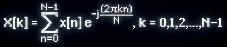
e^-j(2πkn/N) can be thought of as the complex "weight" or amplitude of the kth frequency. In this case, the kth frequency is one whose samples are spread over k rotations over the complex unit circle.

Why use e^iθ over just cosine waves (or sine waves)?

You might ask: Why introduce complex numbers? Why not just correlate with standard cosine waves? This is one thing I initially was confused about.

The problem with a simple cosine wave is that it is phase blind. Let's say your audio signal is a pure sine wave of frequency 3 Hz, correlating it with a Cosine wave of 3 hz results in zero, because they are orthogonal (90 degrees out of phase). The math would wrongly tell you that the frequency doesn't exist.

Complex numbers solve this by using Euler's formula to project the signal against both a cosine (Real axis) and a sine (Imaginary axis) simultaneously. This gives us a 2D "coordinate" for every frequency bin, allowing us to recover the exact alignment:

• Magnitude: sqrt(Real^2 + Imag^2) (Total energy)
• Phase: atan(Imag, Real) (The starting angle)

With atan, we can precisely calculate the phase shift required to reconstruct the original signal.

Programming the naive DFT - Starting with a Single Bin

First, we define a function to calculate the energy for just one specific frequency (k). This projects the signal onto a specific sine/cosine wave.

struct Complex { float Real; float Imag; };

// Calculate DFT bin for a specific frequency index K
Complex DftBin(const std::vector& Signal, int K) {
    int N = Signal.size();
    Complex Xk = {0.0f, 0.0f};
    
    for (int n = 0; n < N; n++) {
        // Euler's Formula: e^-ix = cos(x) - i*sin(x)
        float theta = -2.0f * PI * K * n / N;
        
        Xk.Real += Signal[n] * std::cos(theta);
        Xk.Imag += Signal[n] * std::sin(theta);
    }
    return Xk;
}

Programming the Full Spectrum DFT

To build the complete frequency spectrum, we simply iterate through every possible integer frequency from 0 to N-1, collecting the results into a vector.

// The naive O(N^2) DFT implementation
std::vector FullDFT(const std::vector& Signal) {
    int N = Signal.size();
    std::vector Spectrum;
    
    // Iterate through every frequency bin K
    for (int k = 0; k < N; k++) {
        Spectrum.push_back(DftBin(Signal, k));
    }
    return Spectrum;
}

Why is k integral exactly?

You might wonder why k is always an integer (0, 1, 2...) rather than a decimal like 2.5.

The DFT assumes the signal of length N is periodic. For the math to work orthogonally, we are testing how many complete cycles fit exactly into our window of N samples.

If k=1, the wave fits once. If k=2, it fits twice. These integer frequencies form a basis - a coordinate system for the signal space. If we used non-integers, our "coordinates" would overlap, breaking the clean decomposition of the signal.

Visualizing the Wrap using a "Winding Machine"

The core mechanic of the DFT is "wrapping" the signal around the origin. When the wrap rate matches a frequency in the signal, the points line up.

Notice how the "Center of Mass" (the red dot) stays near the center (0,0) for most frequencies. However, when the winding frequency matches the signal's frequency, the graph aligns to the right, pulling the center of mass away from the origin. That distance is the magnitude of the frequency.

Ok, now what if my frequency isn't integral?

Real-world audio doesn't care about our integer bins. A guitar string might vibrate at a frequency that lands at k = 5.4.

When the frequency doesn't complete a full cycle within the window N, the endpoints don't match up. This creates a sharp discontinuity if we were to loop the signal.

The DFT interprets this sharp jump as a burst of energy across many frequencies. Consequently, the energy "leaks" from the main frequency bin into its neighbors. This is called Spectral Leakage.

The Short Time Fourier Transform

The standard DFT has a fatal flaw: it is timeless.

If you take the DFT of an entire song, the math will tell you exactly which notes were played, but it cannot tell you when they were played. A C-major chord played at the beginning looks mathematically identical to one played at the end.

To solve this, we don't process the whole signal at once. Instead, we chop the signal into small, overlapping blocks (or "windows") and run the DFT on each block individually. This technique, the STFT, allows us to see how frequencies evolve over time.

The Periodicity Assumption

When we slice audio into blocks for the STFT, the math inherently assumes that each small block repeats infinitely. However, because our cuts are arbitrary, the end of the block rarely lines up with the start.

This mismatch creates a sharp discontinuity - a "cliff" - every time the loop repeats. To the DFT, this cliff looks like a burst of high-frequency noise, muddying our analysis.

The Hann Filter

To fix the cliff, we cheat. We multiply the block by a "Window Function" like the Hann Filter before processing it. This shapes the audio into a smooth bell curve, tapering the jagged edges down to zero. We can then undo this transformation while taking the IDFT (inverse transform).

Now, when the blocks repeat, the start and end points meet perfectly at silence. By making the signal periodic and continuous, we get a clean, accurate frequency reading.

Time vs Frequency Res Tradeoff

Nature *demands* a price. We encounter a limit similar to the Heisenberg Uncertainty Principle.

• To get precise Time information, we need very short windows.
• To get precise Frequency information, we need very long windows (larger N).

If we shrink our window to pinpoint the exact millisecond a drum hit, our frequency bins become wide and coarse (poor resolution). If we widen the window to distinguish between 440Hz and 441Hz, we smear the event out over time.

"We are forever trapped between knowing when it happened, and knowing exactly what it was."

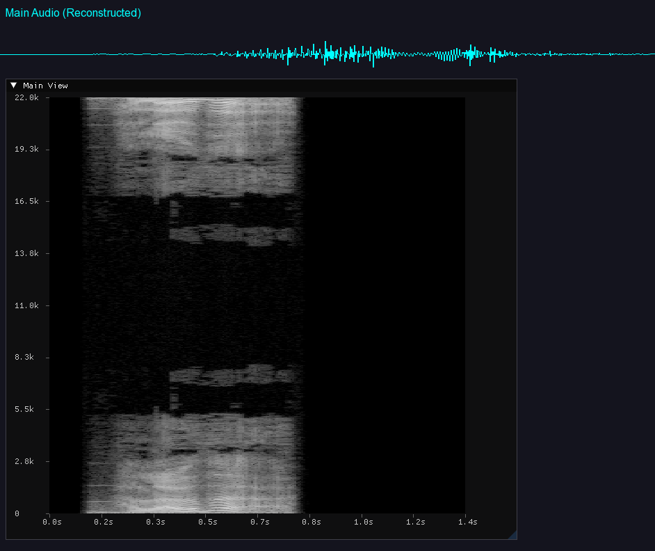
Generating audio spectrum

Now that we can generate frequency data for set time intervals via the STFT, we can plot them sequentially. By mapping Time to the X-axis and Frequency to the Y-axis, we obtain a heat map of the sound.

Adjusting the visual scales and mapping amplitude to color intensity allows us to "Look" at our audio from a new perspective. We can visually distinguish the transient snap of a snare drum from the steady harmonic layers of a synthesizer.

Fig 7. Visualizing the Frequency Domain

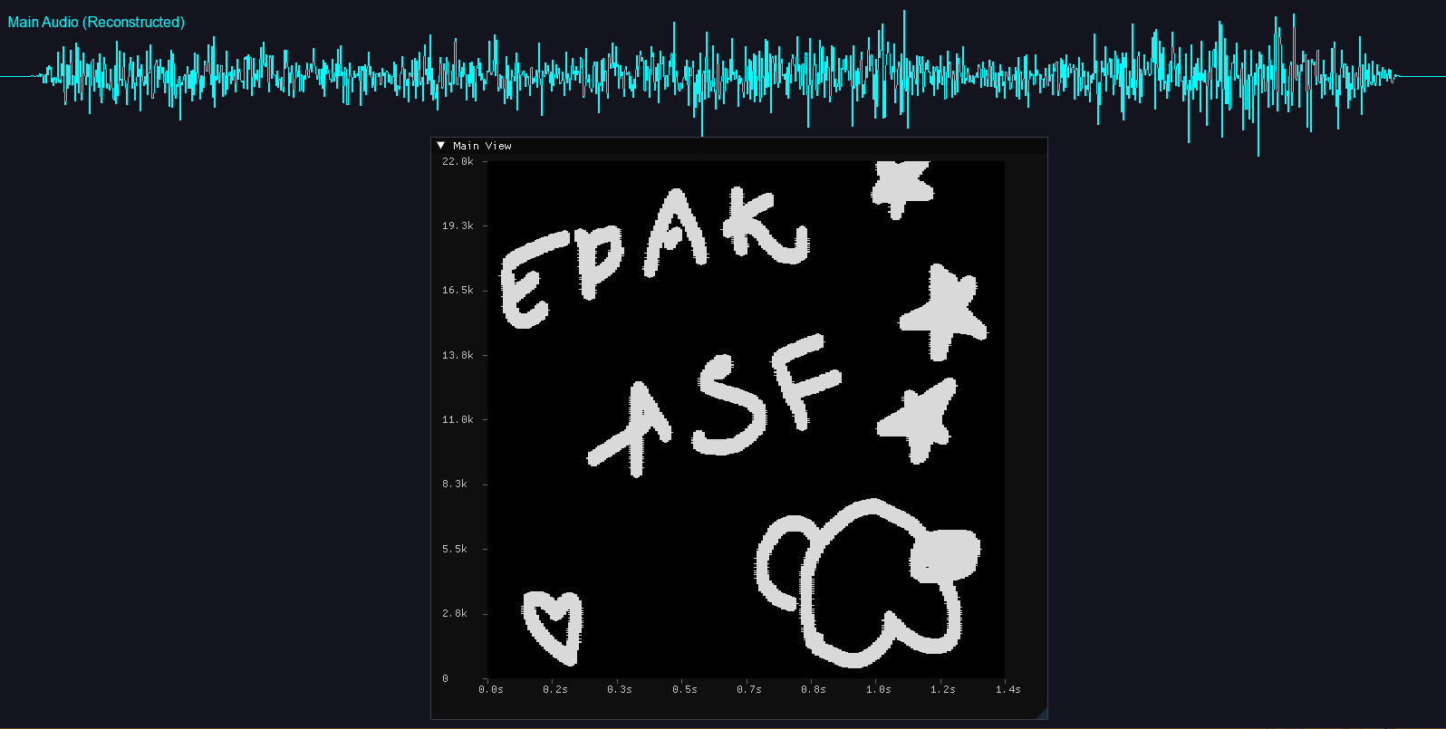
Drawing Audio!

The transformation is bidirectional. We can add a brush tool and suddenly we're able to draw audio directly onto the spectrogram.

By painting onto the frequency canvas and running the Inverse DFT (IDFT), we convert the image back into sound waves. It is surprisingly effective; drawing a shape that "looks" like a chirp generally sounds like a chirp. We can essentially sculpt sound like clay.

Fig 8. Inverse FFT Painting

Conclusion

It is genuinely amazing that we can effectively "paint" sound. By simply changing the "perspective" with which we look at audio, we can do so much more.

You can check out the full source code for this project here: AudioAnalyzer.

And a video that demonstrates it : Youtube.